
Many researchers favor repeated measures designs because they allow the detection of within-person change over time and typically have higher statistical power than cross-sectional designs. However, the plethora of inputs needed for repeated measures designs can make sample size selection, a critical step in designing a successful study, difficult. Using a dental pain study as a driving example, we provide guidance for selecting an appropriate sample size for testing a time by treatment interaction for studies with repeated measures. We describe how to (1) gather the required inputs for the sample size calculation, (2) choose appropriate software to perform the calculation, and (3) address practical considerations such as missing data, multiple aims, and continuous covariates.
Selecting an appropriate sample size is a crucial step in designing a successful study. A study with an insufficient sample size may not have sufficient statistical power to detect meaningful effects and may produce unreliable answers to important research questions. On the other hand, a study with an excessive sample size wastes resources and may unnecessarily expose study participants to potential harm. Choosing the right sample size increases the chance of detecting an effect, and ensures that the study is both ethical and cost-effective.
Repeated measures designs are widely used because they have advantages over cross-sectional designs. For instance, collecting repeated measurements of key variables can provide a more definitive evaluation of within-person change across time. Moreover, collecting repeated measurements can simultaneously increase statistical power for detecting changes while reducing the costs of conducting a study. In spite of the advantages over cross-sectional designs, repeated measures designs complicate the crucial process of selecting a sample size. Unlike studies with independent observations, repeated measurements taken from the same participant are correlated, and the correlations must be accounted for in calculating the appropriate sample size. Some current software packages used for sample size calculations are based on oversimplified assumptions about correlation patterns. As discussed later in the paper, oversimplified assumptions can give investigators false confidence in the chosen sample size. In addition, some current software may require programming skills that are beyond the resources available to many researchers.
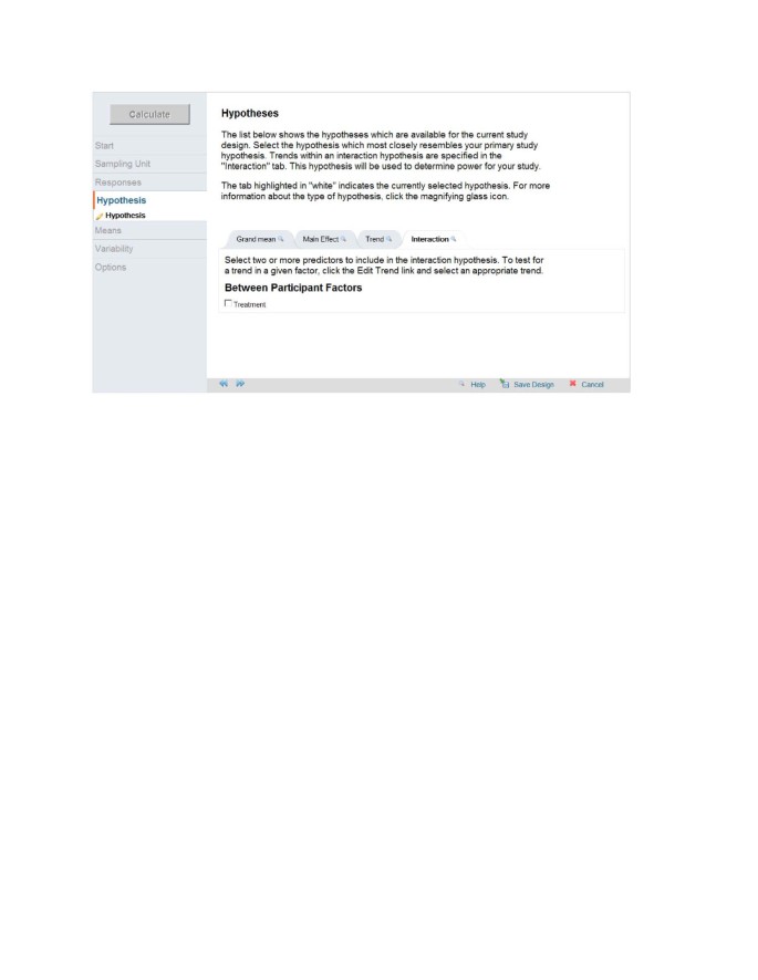
In the present article, we describe methods for gathering the information required for selecting a sample size for studies with repeated measurements of normally distributed continuous responses. We also illustrate the process of sample size selection by working through an example with repeated measurements of pain memory, using the web-based power and sample size program GLIMMPSE.
For the sake of brevity, we will not elaborate on the fundamental question of choosing a data analysis method. Although statistical consulting will have value at any stage of research, the earlier stages of planning a study profit most from consulting. We assume the iterative process of choosing and refining the research goals, the primary outcomes, and the sampling plan has succeeded. In turn, we also assume that an appropriate analysis plan has been selected, which sets the stage for sample size selection.
One of the first steps in computing a sample size is to select a power analysis method that adequately aligns with the data analysis method [1]. As an example, consider a study in which a researcher plans to test whether veterans and non-veterans respond similarly to a drug. The researcher plans to control for both gender and age. The planned data analysis is an analysis of covariance (ANCOVA), with age as the covariate. In this case, a sample size calculation based on a two-group t-test would be inappropriate, since the planned data analysis is not a t-test. Misalignment between the design used for sample size calculations and the design used for data analysis can lead to a sample size that is either too large or too small [1], contributing to inconclusive findings.
In practice, mixed models have become the most popular method for analyzing repeated measures and longitudinal data. However, validated power and sample size methods exist only for a limited class of mixed models [2]. In addition, most of these methods are based on approximations, and make simple assumptions about the study design. In some cases, the planned data analysis has no published power analysis methods aligned with the data analysis. One possible method for finding reliable power or sample size when no power formulas are available is to conduct a computer simulation study. We recommend using appropriate software that has been tested and validated whenever it is available. Packaged software has the advantages of requiring less programming and less statistical sophistication.
Based on the current state of knowledge, we recommend using power methods developed for multivariate models to calculate sample size for studies using common mixed models for data analysis. For carefully built mixed models [3, 4], power methods developed for multivariate models provide the best available power analysis. Technical background can be found in Muller et al. [1], Muller et al. [5], and Johnson et al. [6]. Another option is to use the large sample approximation for power described by Liu and Liang. They proposed a method to compute sample sizes for studies with correlated observations based on the generalized estimating equation (GEE1) approach [7].
When planning a study with repeated measures, scientists must specify variance and correlation patterns among the repeated measurements. Failing to specify variance and correlation patterns aligned with the ones that will be seen in the proposed study can lead to incorrect power analysis [1].
The simplest variance pattern assumes equal variance among the repeated measurements. For example, measuring children’s mathematical achievement within a classroom makes it reasonable to assume equal variability across children, on average. In contrast, measuring mathematical achievement from the same children in grades 6, 7, and 8 could plausibly lead to increasing variability, decreasing variability, or stable variability. Variability in performance on a test of a certain skill could decrease across the grades due to a stable acquisition of the skill. On the other hand, variability of standardized test scores could remain unchanged due to careful test construction by the test developers. Repeated measurements of some variables may have any possible pattern of variance. For example, depending on the experimental condition, the metabolite concentrations in blood might increase, decrease, or remain unchanged across time.
Regarding correlation patterns, it is useful to think of them as having four types, in increasing complexity: (1) zero correlations (independent observations), (2) equal correlations, (3) rule-based patterns, and (4) unstructured correlations (no specific pattern).
The simplest model of correlations assumes a constant correlation, often referred to as an intra-class correlation, among all observations. If each observation records some aspect of a child’s performance within a classroom, then assuming a common correlation among any two children seems reasonable. In contrast, if the same child is measured in grades 6, 7, and 8, we expect the correlation between grades 6 and 8 to be lower than the correlation between grades 6 and 7. Correlations among the repeated measures from a single participant usually vary across time in a smooth and orderly fashion. Measurements taken close in time are usually more correlated than measurements taken farther apart in time.
Many rule-based patterns of correlation have been developed in the context of time series models. One common example of a rule-based pattern is the first-order autoregressive (AR1), a special case of the linear exponent first-order autoregressive (LEAR) family [8]. The AR1 and the more general LEAR patterns assume that correlations among repeated measures decline exponentially with time or distance. For example, in pain studies that examine the effects of interventions on patients’ memory of pain after treatment, the correlations among the measurements of pain memory from the same patient normally decrease over time. The relationship between memory of pain and passage of time can be modeled using the LEAR structure.
The unstructured correlation pattern assumes there are no particular correlation patterns among the repeated measures. Each correlation between any two repeated measurements may be unique. An unstructured correlation pattern requires knowing p × (p−1)/2 distinct correlations, with p being the number of repeated measures.
It is usually assumed that all participants in a study show the same pattern of correlation. Statistical methods are available to allow different correlation patterns among study participants. Although rarely used, a conscientious data analysis should include a meaningful evaluation of the validity of homogeneity of correlation pattern across groups of participants.
Each of the correlation patterns has limitations. Structured correlation patterns reflect special assumptions about the correlations among the repeated measures. The assumptions introduce the risk of choosing a pattern that is too simple, which can falsely inflate the type I error rate [3]. For example, the equal correlation pattern assumes that any pair of observations has the same correlation, no matter how far apart in time they fall. On the other hand, choosing an unstructured correlation pattern can be impractical because it requires estimating more parameters than the data support, which leads to a failure to converge. A flexible structure, such as the LEAR pattern, often provides the best compromise between too little complexity (equal correlation) and too much (unstructured correlation).
We illustrate how to find valid inputs for sample size calculations with an example drawn from a clinical study that used repeated measures of dental pain as the outcomes. The investigator plans to randomize the study participants to one of two groups, either control or treatment. Knowledge of the pain scale makes it reasonable to assume the data follow a normal distribution. The inputs needed to compute a sample size are (1) α, the Type I error rate, (2) the predictors implied by the design, (3) the target hypothesis being tested, (4) the difference in the pattern of means for which good power is being sought, (5) the variances of the response variables, and (6) the correlations among the response variables (Table 1). Finding the last three items in the list requires most of the effort.
The main response variable of interest is memory of pain. It is a continuous variable that ranges from 0 to 5.0, with 0 meaning no pain remembered and 5.0 meaning maximum pain remembered [14]. Memory of pain will be assessed immediately after the dental procedure (Pain0), one week later (Pain1), six months later (Pain2), and twelve months later (Pain3). Pain0 will be measured in the clinic. Pain1, Pain2, and Pain3 will be measured through telephone interviews. The spacing in repeated measures is chosen based on the investigators’ knowledge of how pain memory changes over time.
The primary predictor of interest is the intervention (i.e., the audio instruction for participants to use a sensory focus during their respective dental procedures). In the new study, the Iowa Dental Control Index (IDCI) will be used to categorize and select patients [19]. Only patients with a high desire for control and low felt control will be recruited. Patients in this group will be selected and randomly assigned to either intervention or no intervention. Those in the intervention group will listen to automated audio instructions, in which they are told to pay close attention only to the physical sensations in their mouth [14]. Patients in the no-intervention group will listen to automated audio instructions on a neutral topic to control for media and attention effects. As in earlier studies, appropriate manipulation checks will be used [14].
Once the goals and the variables are specified, the next step is to specify the variance and correlation patterns among the repeated measures. In our case, the variance of difference between Pain0 was 0.96 in a previous study conducted by the investigators [14]. This variance of difference can be directly used as an estimate for the variances of the pain memory measures, Var(Paini). As for the required correlations, 6 correlation values need to be estimated since there are 4 repeated measurements (Table 2). Prior research reports that the correlation between experienced pain and 1-week memory of pain is 0.60, and the correlation between experienced pain and 18-month memory of pain is 0.39 [18]. Therefore, it is reasonable to believe that the correlation between Pain0 and Pain1 is 0.60. In addition, since the investigators believe that the correlations decay smoothly across time, it is reasonable to assume the Pain0 - Pain1, Pain0 - Pain2, and Pain0 - Pain3 correlations are all larger than 0.39. Based on the trend of decay and the restrictive lower bound of 0.39, the investigators estimate that the Pain0 - Pain1, Pain0 - Pain2, and Pain0 - Pain3 correlations are approximately 0.6, 0.5, and 0.4, respectively (second column in Table 2). Following a similar thought process, the investigators estimate that the Pain1 - Pain2, Pain1 - Pain3, and Pain2 - Pain3 correlations are approximately 0.45, 0.40, and 0.45, respectively (Table 2).
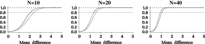
Results from the power analysis are summarized in Figure 3. The y-axis is the power and the x-axis is the mean difference among the Paini measurements (e.g., Pain2 - Pain1). As seen in Figure 3, for a given desired power, the minimum detectable mean difference decreases as sample size increases. The investigators specified a minimal change in pain that they deem clinically important as a difference of 1.2 between the pain measures. A sample size of 40 patients per group, or a total of 80 patients, would give a power of at least 0.8 for testing the hypothesis of whether there is a time × intervention interaction.
Power analysis for studies with repeated measures can be complicated. It often involves solving a problem with many possible answers, such as specifying the variance and correlation patterns among the repeated measurements. Therefore, we recommend consulting with a statistician, if possible, when there are any unclear issues. The online sample size tool Glimmpse is designed such that it guides scientists through power analysis by asking questions about the study design. In the rest of this section, we provide additional practical advice on issues related to power analysis.
One limitation of the power analysis method based on general linear multivariate models is that it is a calculation for complete cases. In a complete case analysis, all repeated measurements on the same participant must be available. However, in longitudinal studies involving human participants, investigators often end up with missing data due to missed visits. One simple strategy to account for expected missing data is to propose an expected attrition rate, and then recruit more people accordingly. In our driving example, the investigators expect a maximum of 20% attrition for the one-year-long study, based on previous experiences with similar research projects. Therefore, they need to collect data for 20% more participants in order to achieve the desired power. On the other hand, this method does not consider partial information that might be obtained from participants with missing visits or dropout participants. There are sample size methods developed for these scenarios, but discussing them is out of the scope of this article [20]. Furthermore, as always, the possibility of non-randomly missing data must be carefully examined by checking the study design and data collection procedures once the data have been collected.
Due to cost and ethical issues, scientists often want to test more than one hypothesis in a study. Each power analysis must be based on one specific hypothesis using a pre-planned data analysis method. With a modest number of primary analyses, a simple Bonferroni correction is typically applied to help control the Type I error rate. For example, with 4 primary hypotheses, a Type I error rate of α = 0.05 ÷ 4 = 0.0125 would be used. Having conducted 4 power analyses leads to 4 different power values or ideal sample sizes. In the absence of time, cost, and ethical concerns, the scientist may choose the largest sample size to guarantee power for all 4 tests.
In addition to categorical variables, continuous variables are sometimes included in studies as predictors or baseline covariates. A baseline covariate is the first measurement (before treatment) of a continuous response measured repeatedly over time. It is included as a predictor variable to control for differences in the starting values of the response. Using a baseline covariate that controls a large proportion of the variance of the response increases the statistical power of the data analysis, but also complicates the calculation of sample size. However, current knowledge of the closed form approximation covers only sample size and power calculation in general linear multivariate models with a single, continuous, normally distributed predictor variable [13]. Glueck and Muller reviewed the limited approximate power methods that are available for adjusting for covariates [13].
Using a repeated measures design improves efficiency and allows testing a time × treatment interaction. In practice, the critical task of selecting a sample size for studies with repeated measures can be daunting. In this article, we described a practical method for selecting a sample size for repeated measures designs and provided an example. In addition, we gave practical advice for addressing potential problems and complications.
Yi Guo, Henrietta Logan, and Keith Muller’s support included NIH/NIDCR 1R01DE020832-01A1 and NIH/NIDCR U54-DE019261. Deborah Glueck’ support included NIH/NIDCR 1R01DE020832-01A1.